Think about a signal, lets say a sine with 5Hz frequency and a sine with 15Hz of frequency with amplitudes of 0.8 and 0.4. They look like this (black and red) and combined like the green one in following figure.
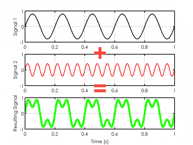
top: y(t)=0.8 sin(2π 5 t), middle: y(t)=0.4 sin(2π 15 t), bottom: mix of both sine wave signals
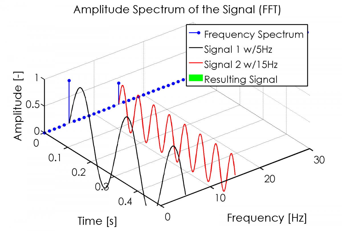
So, how about the Frequency Domain of these signals? Looks like a FFT (=Discrete Fast Fourier Transform) does the right thing for us, right?
Connection between time and frequency domain of a signal
CC-BY-SA2.0
Matlab Code of this FFT Animation
%% Animation zum Zusammenhang zwischen Signal im Zeit und Frequenzbereich
% Paul Balzer
% Motorblog | www.cbcity.de

%% Signal generieren
%
dt = 0.001;
t=0:dt:1;

f1 = 5;
s1 = 0.8*sin(2*pi*f1*t);

f2 = 15;
s2 = 0.4*sin(2*pi*f2*t);

s=s1+s2;

% figure(1)
% subplot(3,1,1)
% plot(t,s1,'-k')
% ylabel('Signal 1')
% ylim([-1 1])
% grid on
%
% subplot(3,1,2)
% plot(t,s2,'-r')
% ylabel('Signal 2')
% ylim([-1 1])
% grid on
%
% subplot(3,1,3)
% plot(t,s,'-g','linewidth',2)
% xlabel('Time [s]')
% ylabel('Resulting Signal')
% ylim([-1 1])
% grid on

%% FFT
%
Y = fft(s);

n = numel(t);            % Anzahl Werte
m = floor(n/2);          % Spektrumbegrenzung aus Nyquist Frequenz

fspec = t.* 1/(dt*n) * 1/dt;    % Frequenzvektor
ampspec = 2.*abs(Y)/n;          % Amplitude

figure(2)
set(gcf,'color',[1 1 1],'position',[10 10 770 520])
hf = stem3(zeros(1,31),fspec(1:31), ampspec(1:31),'fill');
grid on
hold on
hs1 = plot3(t(1:m), f1.*ones(1,m), s1(1:m),'-k');
hs2 = plot3(t(1:m), f2.*ones(1,m), s2(1:m),'-r');

hs = plot3(t(1:m), zeros(1,m), s(1:m),'-g','linewidth',5);

legend('Amplitude Spectrum',['Signal 1 w/' num2str(f1) 'Hz'],...
    ['Signal 2 w/' num2str(f2) 'Hz'],'Resulting Signal',...
    'location','east')

xlabel('Time [s]','fontsize',18)
xlim([0 max(t(1:m))])
ylabel('Frequency [Hz]','fontsize',18)
ylim([0 max(f1,f2)*2])
zlabel('Amplitude [-]','fontsize',18)
box off
set(gca,'fontsize',16)

%% 3D Darstellung erzeugen
%
view(0,0)      % Frequenzspektrum
axis vis3d      % so skalieren, dass beim Drehen nichts mehr skaliert
title('Signal in time Domain','fontsize',18)
drawnow

% GIF erzeugen
mygif = 'Time-2-Frequency-Domain-FFT.gif';
f = getframe(gcf);
[im,map]=rgb2ind(f.cdata,256,'nodither');
imwrite(im,map,mygif,'Delaytime',5,'Loopcount',inf)

for i = 0:0.5:90

    % Smooth View change
    hann=0.5*(1-cos(2*pi*i/90));
    view(90*(3*(i/90)^2-2*(i/90)^3),40*sind(2*i)*hann)

    f = getframe(gcf);
    [im,map]=rgb2ind(f.cdata,256,'nodither');
    imwrite(im,map,mygif,'writemode','append','Delaytime',.02)

end

title('Amplitude Spectrum of the Signal (FFT)','fontsize',18)
set(hs,'visible','off')

for i = -1:.02:0
    zlim([i 1])

    f = getframe(gcf);
    [im,map]=rgb2ind(f.cdata,256,'nodither');
    imwrite(im,map,mygif,'writemode','append','Delaytime',.02)

end

legend('off')
annotation('textbox', [.7 0.0 .1 0.1], 'String', 'CC-BY-SA2.0 Paul Balzer | Motorblog');

drawnow
f = getframe(gcf);
[im,map]=rgb2ind(f.cdata,256,'nodither');
imwrite(im,map,mygif,'writemode','append','Delaytime',5)